
캐글 타이타닉3 - 핸즈온 머신러닝 챕터2 적용
Updated:
아래 포스팅의 jupyter notebook 파일은 아래 링크에서 확인할 수 있습니다.
Hands-on 머신러닝 책의 2장 내용을 캐글-타이타닉 문제에 맞게 재구성한다. 책의 예제는 주택가격을 예측하는 회귀문제이다. 그러나 타이타닉은 생존자를 예측하는 분류문제다. 따라서 모델 성능 지표를 ROC 곡선으로 택한다.
아래 링크의 포스팅과 겹치는 부분은 제외한다.
1. 데이터 불러오기
import numpy as np
import pandas as pd
import matplotlib.pyplot as plt
import seaborn as sns

# 데이터 불러오기
train = pd.read_csv('./train.csv')
test = pd.read_csv('./test.csv')

train_test_data = [train, test]
2. 데이터 전처리
# Sex 전처리
sex_mapping = {"male":0, "female":1}
for dataset in train_test_data:
    dataset['Sex'] = dataset['Sex'].map(sex_mapping)

# SibSp & Parch 전처리
for dataset in train_test_data:
    # 가족수 = 형제자매 + 부모님 + 자녀 + 본인
    dataset['FamilySize'] = dataset['SibSp'] + dataset['Parch'] + 1
    dataset['IsAlone'] = 1

    # 가족수 > 1이면 동승자 있음
    dataset.loc[dataset['FamilySize'] > 1, 'IsAlone'] = 0

# Embarked 전처리
for dataset in train_test_data:
    dataset['Embarked'] = dataset['Embarked'].fillna('S')

embarked_mapping = {'S':0, 'C':1, 'Q':2}
for dataset in train_test_data:
    dataset['Embarked'] = dataset['Embarked'].map(embarked_mapping)

# Name 전처리
for dataset in train_test_data:
    dataset['Title'] = dataset['Name'].str.extract('([\w]+)\.', expand=False)

for dataset in train_test_data:
    dataset['Title'] = dataset['Title'].apply(lambda x: 0 if x=="Mr" else 1 if x=="Miss" else 2 if x=="Mrs" else 3 if x=="Master" else 4)

# Age 결측치 제거
for dataset in train_test_data:
    dataset['Age'].fillna(dataset.groupby("Title")["Age"].transform("median"), inplace=True)

# Fare 결측치 제거
for dataset in train_test_data:
    dataset["Fare"].fillna(dataset.groupby("Pclass")["Fare"].transform("median"), inplace=True)
train.head()
| PassengerId | Survived | Pclass | Name | Sex | Age | SibSp | Parch | Ticket | Fare | Cabin | Embarked | FamilySize | IsAlone | Title | |
|---|---|---|---|---|---|---|---|---|---|---|---|---|---|---|---|
| 0 | 1 | 0 | 3 | Braund, Mr. Owen Harris | 0 | 22.0 | 1 | 0 | A/5 21171 | 7.2500 | NaN | 0 | 2 | 0 | 0 |
| 1 | 2 | 1 | 1 | Cumings, Mrs. John Bradley (Florence Briggs Th... | 1 | 38.0 | 1 | 0 | PC 17599 | 71.2833 | C85 | 1 | 2 | 0 | 2 |
| 2 | 3 | 1 | 3 | Heikkinen, Miss. Laina | 1 | 26.0 | 0 | 0 | STON/O2. 3101282 | 7.9250 | NaN | 0 | 1 | 1 | 1 |
| 3 | 4 | 1 | 1 | Futrelle, Mrs. Jacques Heath (Lily May Peel) | 1 | 35.0 | 1 | 0 | 113803 | 53.1000 | C123 | 0 | 2 | 0 | 2 |
| 4 | 5 | 0 | 3 | Allen, Mr. William Henry | 0 | 35.0 | 0 | 0 | 373450 | 8.0500 | NaN | 0 | 1 | 1 | 0 |
2.1 min-max scaling
min-max scaling은 데이터의 크기를 0~1 사이로 조절한다. 내용과 코드에 대한 설명은 아래 링크를 참조하자.
from sklearn.preprocessing import MinMaxScaler

scaler = MinMaxScaler()
for dataset in train_test_data:
    array = dataset['Age'].values.reshape(-1,1) # 2D array로 변환
    scaler.fit(array) # 스케일링에 필요한 값(최소값, range 등) 계산
    dataset['AgeScale'] = pd.Series(scaler.transform(array).reshape(-1)) # 스케일링 후 series로 추가
2.2 standardization
표준화는 연속변수를 정규분포의 Z변수에 대응시킨다. 설명은 아래 링크 참조.
from sklearn.preprocessing import StandardScaler

scaler = StandardScaler()
for dataset in train_test_data:
    array = dataset[['Fare']] # 한 줄짜리 DataFrame
    scaler.fit(array)
    dataset['FareScale'] = pd.Series(scaler.transform(array).reshape(-1))
min-max 스케일링과 마찬가지로 array에는 2차원 배열이 저장되어야 한다. dataset['Fare']는 series로써 1차원 배열이다. 그러나 dataset[['Fare']]는 모양은 똑같아도 Dataframe이다. Dataframe은 그 자체로 2차원 배열에 해당하므로 fit() 메서드를 이용할 수 있다.
train.head()
| PassengerId | Survived | Pclass | Name | Sex | Age | SibSp | Parch | Ticket | Fare | Cabin | Embarked | FamilySize | IsAlone | Title | AgeScale | FareScale | |
|---|---|---|---|---|---|---|---|---|---|---|---|---|---|---|---|---|---|
| 0 | 1 | 0 | 3 | Braund, Mr. Owen Harris | 0 | 22.0 | 1 | 0 | A/5 21171 | 7.2500 | NaN | 0 | 2 | 0 | 0 | 0.271174 | -0.502445 |
| 1 | 2 | 1 | 1 | Cumings, Mrs. John Bradley (Florence Briggs Th... | 1 | 38.0 | 1 | 0 | PC 17599 | 71.2833 | C85 | 1 | 2 | 0 | 2 | 0.472229 | 0.786845 |
| 2 | 3 | 1 | 3 | Heikkinen, Miss. Laina | 1 | 26.0 | 0 | 0 | STON/O2. 3101282 | 7.9250 | NaN | 0 | 1 | 1 | 1 | 0.321438 | -0.488854 |
| 3 | 4 | 1 | 1 | Futrelle, Mrs. Jacques Heath (Lily May Peel) | 1 | 35.0 | 1 | 0 | 113803 | 53.1000 | C123 | 0 | 2 | 0 | 2 | 0.434531 | 0.420730 |
| 4 | 5 | 0 | 3 | Allen, Mr. William Henry | 0 | 35.0 | 0 | 0 | 373450 | 8.0500 | NaN | 0 | 1 | 1 | 0 | 0.434531 | -0.486337 |
2.3 one-hot encoding
one-hot encoding은 하나의 데이터에 하나의 벡터를 대응시키는 변환이다. 대응되는 벡터는 하나의 성분만 1이고 나머지 성분은 0인 n차원 벡터이다. 범주형 데이터를 숫자로 변환할 때 주로 이용한다.
from sklearn.preprocessing import OneHotEncoder

encoder = OneHotEncoder()
category = train[['Sex','Title']]
onehot = encoder.fit_transform(category)
onehot
<891x7 sparse matrix of type '<class 'numpy.float64'>'
	with 1782 stored elements in Compressed Sparse Row format>
MinMaxScaler, StandardScaler와 마찬가지로 OneHotEncoder 역시 fit() 메서드는 2차원 배열을 받는다. 따라서 category에 변환하고 싶은 열들만 추려 DataFrame으로 저장한다.
출력 결과는 희소행렬(Sparse matrix)이다. 눈에 보이게끔 하고 싶다면 dataframe으로 바꾸면 된다.
pd.DataFrame(onehot.toarray())
| 0 | 1 | 2 | 3 | 4 | 5 | 6 | |
|---|---|---|---|---|---|---|---|
| 0 | 1.0 | 0.0 | 1.0 | 0.0 | 0.0 | 0.0 | 0.0 |
| 1 | 0.0 | 1.0 | 0.0 | 0.0 | 1.0 | 0.0 | 0.0 |
| 2 | 0.0 | 1.0 | 0.0 | 1.0 | 0.0 | 0.0 | 0.0 |
| 3 | 0.0 | 1.0 | 0.0 | 0.0 | 1.0 | 0.0 | 0.0 |
| 4 | 1.0 | 0.0 | 1.0 | 0.0 | 0.0 | 0.0 | 0.0 |
| ... | ... | ... | ... | ... | ... | ... | ... |
| 886 | 1.0 | 0.0 | 0.0 | 0.0 | 0.0 | 0.0 | 1.0 |
| 887 | 0.0 | 1.0 | 0.0 | 1.0 | 0.0 | 0.0 | 0.0 |
| 888 | 0.0 | 1.0 | 0.0 | 1.0 | 0.0 | 0.0 | 0.0 |
| 889 | 1.0 | 0.0 | 1.0 | 0.0 | 0.0 | 0.0 | 0.0 |
| 890 | 1.0 | 0.0 | 1.0 | 0.0 | 0.0 | 0.0 | 0.0 |
891 rows × 7 columns
위의 예시를 바탕으로 train, test 데이터에 대해 one-hot encoding을 진행한다.
encoder = OneHotEncoder()
train_test_data2=[]

for dataset in train_test_data:
    category = dataset[['Sex', 'Title', 'Embarked', 'IsAlone', 'Pclass']]
    onehot = encoder.fit_transform(category)
    df = pd.DataFrame(onehot.toarray())
    df2 = pd.concat([dataset, df], axis=1)
    train_test_data2.append(df2)

train = train_test_data2[0]
test = train_test_data2[1]
train.info()
<class 'pandas.core.frame.DataFrame'>
RangeIndex: 891 entries, 0 to 890
Data columns (total 32 columns):
 #   Column       Non-Null Count  Dtype
---  ------       --------------  -----
 0   PassengerId  891 non-null    int64
 1   Survived     891 non-null    int64
 2   Pclass       891 non-null    int64
 3   Name         891 non-null    object
 4   Sex          891 non-null    int64
 5   Age          891 non-null    float64
 6   SibSp        891 non-null    int64
 7   Parch        891 non-null    int64
 8   Ticket       891 non-null    object
 9   Fare         891 non-null    float64
 10  Cabin        204 non-null    object
 11  Embarked     891 non-null    int64
 12  FamilySize   891 non-null    int64
 13  IsAlone      891 non-null    int64
 14  Title        891 non-null    int64
 15  AgeScale     891 non-null    float64
 16  FareScale    891 non-null    float64
 17  0            891 non-null    float64
 18  1            891 non-null    float64
 19  2            891 non-null    float64
 20  3            891 non-null    float64
 21  4            891 non-null    float64
 22  5            891 non-null    float64
 23  6            891 non-null    float64
 24  7            891 non-null    float64
 25  8            891 non-null    float64
 26  9            891 non-null    float64
 27  10           891 non-null    float64
 28  11           891 non-null    float64
 29  12           891 non-null    float64
 30  13           891 non-null    float64
 31  14           891 non-null    float64
dtypes: float64(19), int64(10), object(3)
memory usage: 222.9+ KB
3. 모델 선택 & 학습
# 전처리가 끝난 특성들 제거
drop_column = ['Name', 'Age', 'SibSp', 'Parch', 'Ticket', 'Fare', 'Cabin', 'FamilySize', 'Pclass', 'Sex', 'Title', 'IsAlone', 'Embarked']

train.drop(drop_column, axis=1, inplace=True)
test.drop(drop_column, axis=1, inplace=True)
train.info()
<class 'pandas.core.frame.DataFrame'>
RangeIndex: 891 entries, 0 to 890
Data columns (total 19 columns):
 #   Column       Non-Null Count  Dtype
---  ------       --------------  -----
 0   PassengerId  891 non-null    int64
 1   Survived     891 non-null    int64
 2   AgeScale     891 non-null    float64
 3   FareScale    891 non-null    float64
 4   0            891 non-null    float64
 5   1            891 non-null    float64
 6   2            891 non-null    float64
 7   3            891 non-null    float64
 8   4            891 non-null    float64
 9   5            891 non-null    float64
 10  6            891 non-null    float64
 11  7            891 non-null    float64
 12  8            891 non-null    float64
 13  9            891 non-null    float64
 14  10           891 non-null    float64
 15  11           891 non-null    float64
 16  12           891 non-null    float64
 17  13           891 non-null    float64
 18  14           891 non-null    float64
dtypes: float64(17), int64(2)
memory usage: 132.4 KB
test.info()
<class 'pandas.core.frame.DataFrame'>
RangeIndex: 418 entries, 0 to 417
Data columns (total 18 columns):
 #   Column       Non-Null Count  Dtype
---  ------       --------------  -----
 0   PassengerId  418 non-null    int64
 1   AgeScale     418 non-null    float64
 2   FareScale    418 non-null    float64
 3   0            418 non-null    float64
 4   1            418 non-null    float64
 5   2            418 non-null    float64
 6   3            418 non-null    float64
 7   4            418 non-null    float64
 8   5            418 non-null    float64
 9   6            418 non-null    float64
 10  7            418 non-null    float64
 11  8            418 non-null    float64
 12  9            418 non-null    float64
 13  10           418 non-null    float64
 14  11           418 non-null    float64
 15  12           418 non-null    float64
 16  13           418 non-null    float64
 17  14           418 non-null    float64
dtypes: float64(17), int64(1)
memory usage: 58.9 KB
# 훈련을 위한 train, target 분할
drop_column2 = ['PassengerId', 'Survived']
train_data = train.drop(drop_column2, axis=1)
target = train['Survived']
3.1 k-fold cross-validation
랜덤 포레스트 모델에 대해 k-겹 교차검증을 진행한다. 교차검증에 대한 설명은 아래 링크 참조.
# 랜덤 포레스트 패키지
from sklearn.ensemble import RandomForestClassifier

# 교차검증 패키지
from sklearn.model_selection import cross_val_predict
cross_val_predict는 train 세트에 대해 교차검증을 수행한다. 그러나 cross_val_score와 달리 평가점수를 반환하지 않고 각 테스트 폴드에서 얻은 예측을 반환한다. 각 테스트 폴드의 합은 전체 훈련 세트와 같다. 따라서 교차검증 수행결과 훈련 세트의 모든 샘플에 대해 예측 결과를 얻게 된다.
clf = RandomForestClassifier()
proba_score = cross_val_predict(clf, train_data, target, cv=5, method='predict_proba')
pd.DataFrame(proba_score)
| 0 | 1 | |
|---|---|---|
| 0 | 0.602500 | 0.397500 |
| 1 | 0.010000 | 0.990000 |
| 2 | 0.350000 | 0.650000 |
| 3 | 0.000000 | 1.000000 |
| 4 | 0.993333 | 0.006667 |
| ... | ... | ... |
| 886 | 0.950000 | 0.050000 |
| 887 | 0.080000 | 0.920000 |
| 888 | 0.900000 | 0.100000 |
| 889 | 0.580000 | 0.420000 |
| 890 | 0.923333 | 0.076667 |
891 rows × 2 columns
3.2 모델 평가
# ROC curve 패키지
from sklearn.metrics import roc_curve
from sklearn.metrics import roc_auc_score
y_score = proba_score[:,1] # 두 번째 열 저장
fpr, tpr, thresholds = roc_curve(target, y_score)

print(thresholds, len(thresholds))

plt.plot(fpr, tpr)
plt.plot([0,1], [0,1], 'k--')
plt.show()
roc_auc_score(target, y_score)
[2.00000000e+00 1.00000000e+00 9.95000000e-01 9.90000000e-01
 9.86067599e-01 9.81666667e-01 9.80000000e-01 9.75086580e-01
 9.70000000e-01 9.60000000e-01 9.52090909e-01 9.51666667e-01
 9.50000000e-01 9.46666667e-01 9.45833333e-01 9.40000000e-01
 9.32000000e-01 9.30000000e-01 9.23333333e-01 9.21666667e-01
 9.20000000e-01 9.10500000e-01 9.10000000e-01 9.06221161e-01
 9.00000000e-01 8.97000000e-01 8.90000000e-01 8.88785714e-01
 8.80000000e-01 8.70809524e-01 8.70000000e-01 8.60000000e-01
 8.54571567e-01 8.50000000e-01 8.47047425e-01 8.40000000e-01
 8.37416084e-01 8.33333333e-01 8.30000000e-01 8.24000000e-01
 8.20000000e-01 8.16515152e-01 8.10000000e-01 7.92166667e-01
 7.90000000e-01 7.80000000e-01 7.70000000e-01 7.69166667e-01
 7.60000000e-01 7.50519120e-01 7.50000000e-01 7.43551759e-01
 7.40000000e-01 7.38500000e-01 7.30000000e-01 7.15000000e-01
 7.00000000e-01 6.90000000e-01 6.80000000e-01 6.70000000e-01
 6.60000000e-01 6.50000000e-01 6.49142857e-01 6.45485570e-01
 6.43333333e-01 6.42628427e-01 6.40000000e-01 6.30000000e-01
 6.20000000e-01 6.10000000e-01 5.95000000e-01 5.80000000e-01
 5.75666667e-01 5.70000000e-01 5.60000000e-01 5.54285714e-01
 5.50000000e-01 5.40000000e-01 5.30000000e-01 5.20000000e-01
 5.16666667e-01 5.12833333e-01 5.10000000e-01 5.00000000e-01
 4.80000000e-01 4.73333333e-01 4.70000000e-01 4.60333333e-01
 4.60000000e-01 4.50000000e-01 4.47833333e-01 4.43333333e-01
 4.40000000e-01 4.35833333e-01 4.30000000e-01 4.10000000e-01
 4.00000000e-01 3.97500000e-01 3.90000000e-01 3.80000000e-01
 3.73305556e-01 3.70000000e-01 3.60000000e-01 3.54333333e-01
 3.50000000e-01 3.40000000e-01 3.34333333e-01 3.30000000e-01
 3.20000000e-01 3.19869048e-01 3.10000000e-01 3.09333333e-01
 3.00000000e-01 2.91666667e-01 2.90000000e-01 2.81861111e-01
 2.80000000e-01 2.71833333e-01 2.70000000e-01 2.60540404e-01
 2.60000000e-01 2.54678571e-01 2.50000000e-01 2.44166667e-01
 2.40000000e-01 2.30000000e-01 2.24000000e-01 2.20000000e-01
 2.13333333e-01 2.10000000e-01 2.10000000e-01 2.00000000e-01
 1.98214286e-01 1.90000000e-01 1.80000000e-01 1.70658786e-01
 1.70000000e-01 1.60000000e-01 1.59166667e-01 1.58333333e-01
 1.50000000e-01 1.49166667e-01 1.48666667e-01 1.45666667e-01
 1.40000000e-01 1.34000000e-01 1.30785714e-01 1.30000000e-01
 1.25000000e-01 1.21666667e-01 1.20000000e-01 1.18702825e-01
 1.12500000e-01 1.10000000e-01 1.07333694e-01 1.01666667e-01
 1.00324287e-01 1.00000000e-01 9.41666667e-02 9.33883894e-02
 9.10000000e-02 9.00000000e-02 8.25000000e-02 8.00000000e-02
 7.66666667e-02 7.50000000e-02 7.19523810e-02 7.08333333e-02
 7.00000000e-02 6.66666667e-02 6.00000000e-02 5.83333333e-02
 5.75000000e-02 5.66666667e-02 5.58333333e-02 5.25000000e-02
 5.23333333e-02 5.00000000e-02 4.75000000e-02 4.08333333e-02
 4.00000000e-02 3.14202172e-02 3.00000000e-02 2.33333333e-02
 2.20000000e-02 2.17777778e-02 2.13096348e-02 2.00000000e-02
 2.00000000e-02 1.83333333e-02 1.66666667e-02 1.54166667e-02
 1.50000000e-02 1.00000000e-02 9.16666667e-03 8.33333333e-03
 7.75000000e-03 7.50000000e-03 6.66666667e-03 5.00000000e-03
 3.75000000e-03 3.33333333e-03 1.11111111e-03 0.00000000e+00] 204
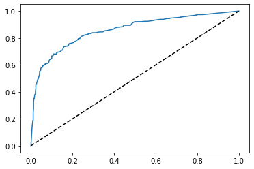
0.8565280840230509
204개의 임계값에 대해 특이도와 민감도를 계산해서 그린 ROC 곡선이다.
4. 모델 파라미터 튜닝
score_list=[]
for i in range(1, 20):
    clf = RandomForestClassifier(max_depth=i, random_state=0, n_jobs=-1)
    y_proba = cross_val_predict(clf, train_data, target, cv=5, method='predict_proba')
    y_score = y_proba[:,1]
    auc = roc_auc_score(target, y_score)
    score_list.append(auc)

score_data_frame = pd.DataFrame(score_list, index=range(1, 20))
score_data_frame
| 0 | |
|---|---|
| 1 | 0.840033 |
| 2 | 0.843069 |
| 3 | 0.847306 |
| 4 | 0.850744 |
| 5 | 0.858717 |
| 6 | 0.862171 |
| 7 | 0.865865 |
| 8 | 0.866533 |
| 9 | 0.869409 |
| 10 | 0.866546 |
| 11 | 0.866395 |
| 12 | 0.863990 |
| 13 | 0.861918 |
| 14 | 0.855740 |
| 15 | 0.859417 |
| 16 | 0.857676 |
| 17 | 0.857268 |
| 18 | 0.857556 |
| 19 | 0.857268 |
max_depth 파라미터를 1~19까지 조절하여 학습시킨 다음 auc를 출력한 결과이다. max_depth=9 일때 점수가 가장 높다.
score_list=[]
for i in range(1, 20):
    clf = RandomForestClassifier(max_depth=9, min_samples_leaf=i,random_state=0, n_jobs=-1)
    y_proba = cross_val_predict(clf, train_data, target, cv=5, method='predict_proba')
    y_score = y_proba[:,1]
    auc = roc_auc_score(target, y_score)
    score_list.append(auc)

score_data_frame = pd.DataFrame(score_list, index=range(1, 20))
score_data_frame
| 0 | |
|---|---|
| 1 | 0.869409 |
| 2 | 0.867172 |
| 3 | 0.869529 |
| 4 | 0.867167 |
| 5 | 0.865172 |
| 6 | 0.864075 |
| 7 | 0.860786 |
| 8 | 0.859833 |
| 9 | 0.858437 |
| 10 | 0.856629 |
| 11 | 0.855772 |
| 12 | 0.855442 |
| 13 | 0.853101 |
| 14 | 0.853178 |
| 15 | 0.853335 |
| 16 | 0.852286 |
| 17 | 0.850973 |
| 18 | 0.849088 |
| 19 | 0.846510 |
max_depth=9로 고정하고 min과 관련된 변수도 조작해본다. min_samples_leaf=3일때 점수가 가장 높으므로 채택한다.
score_list=[]
for i in range(100, 2100, 100):
    clf = RandomForestClassifier(n_estimators=i, max_depth=9, min_samples_leaf=3,random_state=0, n_jobs=-1)
    y_proba = cross_val_predict(clf, train_data, target, cv=5, method='predict_proba')
    y_score = y_proba[:,1]
    auc = roc_auc_score(target, y_score)
    score_list.append(auc)

score_data_frame = pd.DataFrame(score_list, index=range(100, 2100, 100))
score_data_frame
| 0 | |
|---|---|
| 100 | 0.869529 |
| 200 | 0.869777 |
| 300 | 0.870368 |
| 400 | 0.870237 |
| 500 | 0.870679 |
| 600 | 0.870477 |
| 700 | 0.870275 |
| 800 | 0.870328 |
| 900 | 0.870221 |
| 1000 | 0.870413 |
| 1100 | 0.870157 |
| 1200 | 0.870269 |
| 1300 | 0.870429 |
| 1400 | 0.870440 |
| 1500 | 0.870157 |
| 1600 | 0.870280 |
| 1700 | 0.870227 |
| 1800 | 0.870237 |
| 1900 | 0.870205 |
| 2000 | 0.870253 |
n_estimators=500일때 점수가 가장 높다. 확정된 파라미터들로 모델을 다시 학습시켜 제출한다.
# 모델 훈련
clf = RandomForestClassifier(n_estimators=500, max_depth=9, min_samples_leaf=3, random_state=0, n_jobs=-1)
clf.fit(train_data, target)
test_data = test.drop("PassengerId", axis=1)
predict = clf.predict(test_data)

# 예측 결과 저장
submission = pd.DataFrame({
    'PassengerId' : test['PassengerId'],
    'Survived' : predict})

submission.to_csv('submission21_forest_n500_max9_min3.csv', index=False)

Leave a comment